Fallopian tubes data overview

workflowr

• Summary
• Checks
• Past versions

Last updated: 2024-10-19

Checks: 7 0

Knit directory: DEanalysis/

This reproducible R Markdown analysis was created with workflowr (version 1.7.1). The Checks tab describes the reproducibility checks that were applied when the results were created. The Past versions tab lists the development history.

---

R Markdown file: up-to-date

Great! Since the R Markdown file has been committed to the Git repository, you know the exact version of the code that produced these results.

Environment: empty

Great job! The global environment was empty. Objects defined in the global environment can affect the analysis in your R Markdown file in unknown ways. For reproduciblity it’s best to always run the code in an empty environment.

Seed: set.seed(20230508)

The command set.seed(20230508) was run prior to running the code in the R Markdown file. Setting a seed ensures that any results that rely on randomness, e.g. subsampling or permutations, are reproducible.

Session information: recorded

Great job! Recording the operating system, R version, and package versions is critical for reproducibility.

Cache: none

Nice! There were no cached chunks for this analysis, so you can be confident that you successfully produced the results during this run.

File paths: relative

Great job! Using relative paths to the files within your workflowr project makes it easier to run your code on other machines.

Repository version: e612161

Great! You are using Git for version control. Tracking code development and connecting the code version to the results is critical for reproducibility.

The results in this page were generated with repository version e612161. See the Past versions tab to see a history of the changes made to the R Markdown and HTML files.

Note that you need to be careful to ensure that all relevant files for the analysis have been committed to Git prior to generating the results (you can use wflow_publish or wflow_git_commit). workflowr only checks the R Markdown file, but you know if there are other scripts or data files that it depends on. Below is the status of the Git repository when the results were generated:

Ignored files:
    Ignored:    .Rhistory
    Ignored:    .Rproj.user/
    Ignored:    data/.Rhistory

Untracked files:
    Untracked:  .DS_Store
    Untracked:  .gitignore
    Untracked:  analysis/analysis_humanspine.Rmd
    Untracked:  analysis/simulation_donor_effect.Rmd
    Untracked:  data/.DS_Store
    Untracked:  data/10X_DEresult_update.RData
    Untracked:  data/10X_DEresult_update2.RData
    Untracked:  data/10X_Kang_DEresult.RData
    Untracked:  data/10X_inputdata.RData
    Untracked:  data/10X_inputdata_DEresult.RData
    Untracked:  data/10X_inputdata_cpm.RData
    Untracked:  data/10X_inputdata_integrated.RData
    Untracked:  data/10X_inputdata_lognorm.RData
    Untracked:  data/10Xdata_annotate.rds
    Untracked:  data/Bcells.Rmd
    Untracked:  data/Bcellsce.rds
    Untracked:  data/Kang_DEresult.RData
    Untracked:  data/Kang_data.RData
    Untracked:  data/fallopian_tubes.RData
    Untracked:  data/fallopian_tubes_all.RData
    Untracked:  data/human/
    Untracked:  data/human_spine.RData
    Untracked:  data/human_spine_DEresult.RData
    Untracked:  data/mouse/
    Untracked:  data/permutation.RData
    Untracked:  data/permutation13.RData
    Untracked:  data/permutation2.RData
    Untracked:  data/splatter_simulation.RData
    Untracked:  data/splatter_simulation1.RData
    Untracked:  data/splatter_simulation2.RData
    Untracked:  data/splatter_simulation3.RData
    Untracked:  data/vstcounts.Rdata
    Untracked:  figure/

Unstaged changes:
    Modified:   analysis/.Rhistory
    Modified:   analysis/CD14+-Monocytes.Rmd
    Modified:   code/DE_methods.R

Note that any generated files, e.g. HTML, png, CSS, etc., are not included in this status report because it is ok for generated content to have uncommitted changes.

---

These are the previous versions of the repository in which changes were made to the R Markdown (analysis/fallopian_tubes_overview.Rmd) and HTML (docs/fallopian_tubes_overview.html) files. If you’ve configured a remote Git repository (see ?wflow_git_remote), click on the hyperlinks in the table below to view the files as they were in that past version.

File	Version	Author	Date	Message
Rmd	e886219	C-HW	2024-10-14	minor revise sce
html	e886219	C-HW	2024-10-14	minor revise sce

---

Data introduction

For this project, we are analyzing an scRNA-seq dataset that comprises human immune cells. The dataset consists of a total of 57,182 cells contributed by 5 donors, and it includes sequencing data for 29,382 genes. The raw counts represent UMI counts generated using 10X protocols.

In this project, we utilize four distinct assays as inputs.

• Raw counts: This refers to the raw UMI counts generated from 10X protocols without any normalization or adjustments applied.

• (Unused) Seurat normalized counts: This data type represents the counts from each input sample after normalization using the ‘Seurat::NormalizeData(x, normalization.method = “LogNormalize”, scale.factor = 10000)’ function. This normalization method helps to account for differences in library sizes between samples and scales the data by a factor of 10,000.

• Integrated counts: The integrated data refers to the normalized counts after removing batch effects. This assay only contains information for 2000 genes. The purpose of removing batch effects is to minimize any systematic differences introduced by technical variations across different experimental batches.

• CPM counts: CPM stands for Counts Per Million. This assay is obtained by dividing the counts by the sum of library counts and multiplying the result by a million. The CPM values provide a normalized representation of the expression levels, allowing for meaningful comparisons between samples while accounting for differences in library sizes.

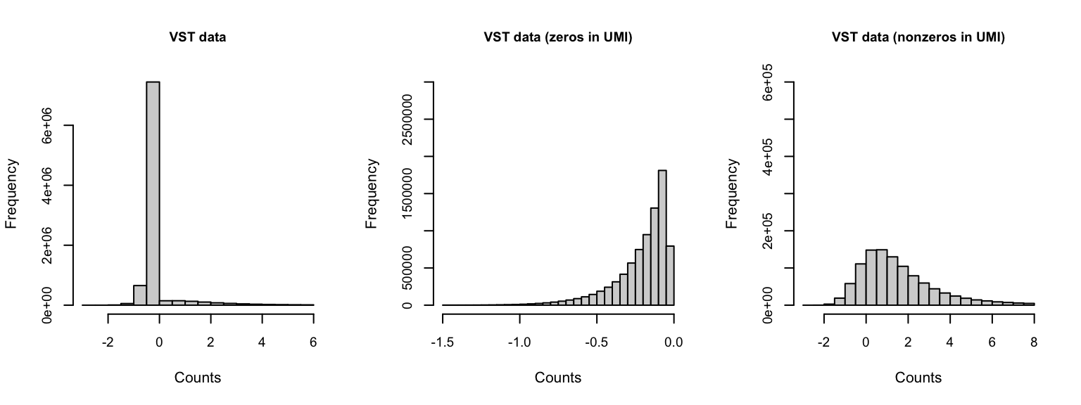
• VST counts: VST (variance stabilizing transformation) is computed via the sctransform package (Hafemeister and Satija 2019), which returns Pearson residuals from a regularized negative binomial regression model that can be interpreted as normalized expression values.

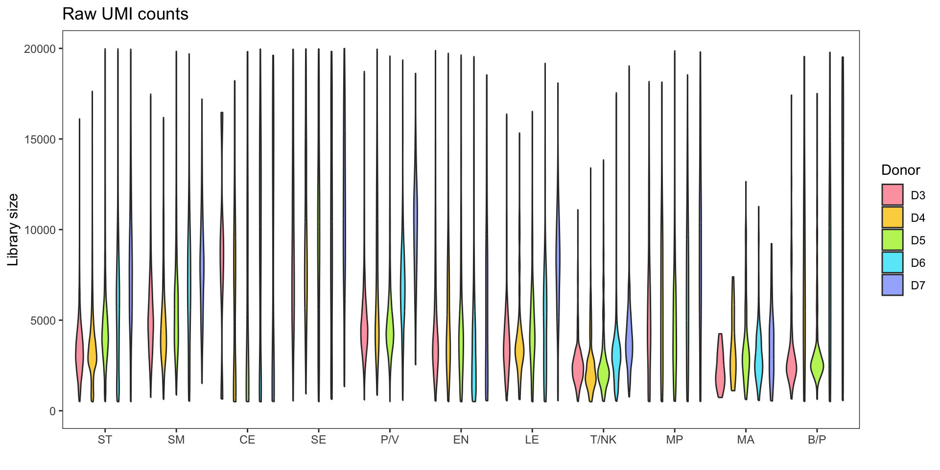
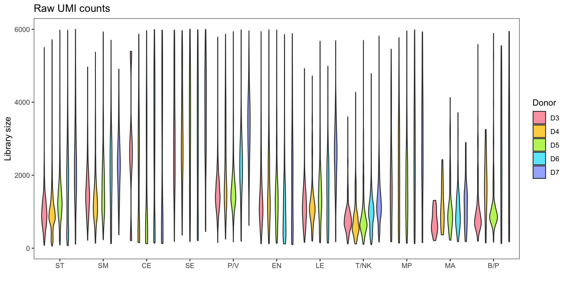
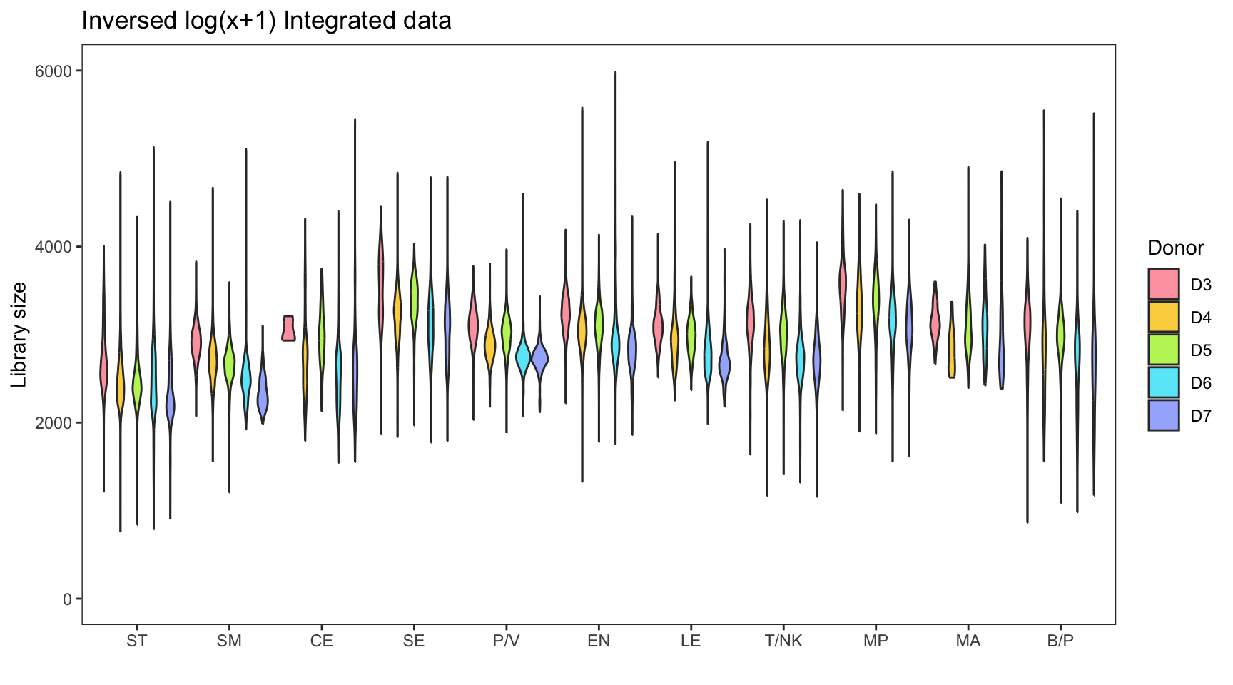
Library size

Before focusing on specific cell types (NK/T), it is important to examine the original dataset, which consists of various cell types. The normalization and integration processes are performed on the entire dataset. It is worth noting that during the preprocessing stage, the specific cell types are typically unknown.

The violin plot presented below illustrates the significant variation in library size among different cell types. This discrepancy can lead to erroneous underestimation or overestimation of gene counts during normalization procedures.

All genes

Past versions of unnamed-chunk-4-1.png

Version	Author	Date
e886219	C-HW	2024-10-14

Genes shown in integrated dataset

Past versions of unnamed-chunk-6-1.png

Version	Author	Date
e886219	C-HW	2024-10-14

Past versions of unnamed-chunk-8-1.png

Version	Author	Date
e886219	C-HW	2024-10-14

Gene expression frequency

Past versions of unnamed-chunk-10-1.png

Version	Author	Date
e886219	C-HW	2024-10-14

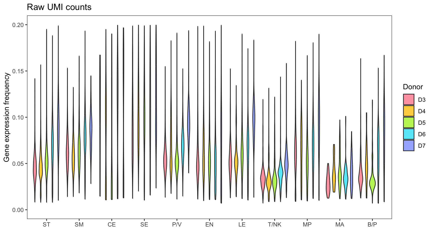
Gene expression distribution

All genes

Past versions of unnamed-chunk-11-1.png

Version	Author	Date
e886219	C-HW	2024-10-14

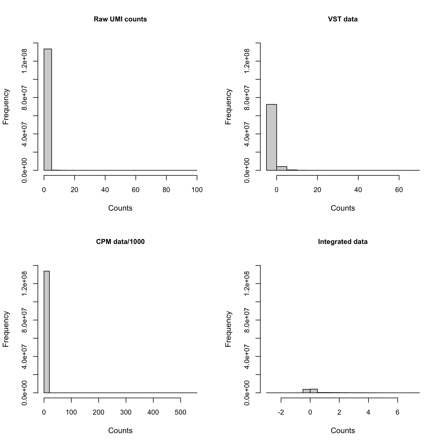
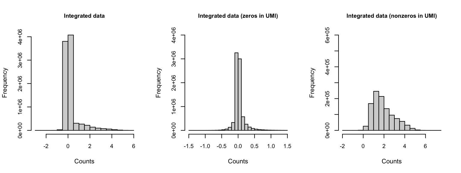
Genes shown in integrated dataset

Past versions of unnamed-chunk-12-1.png

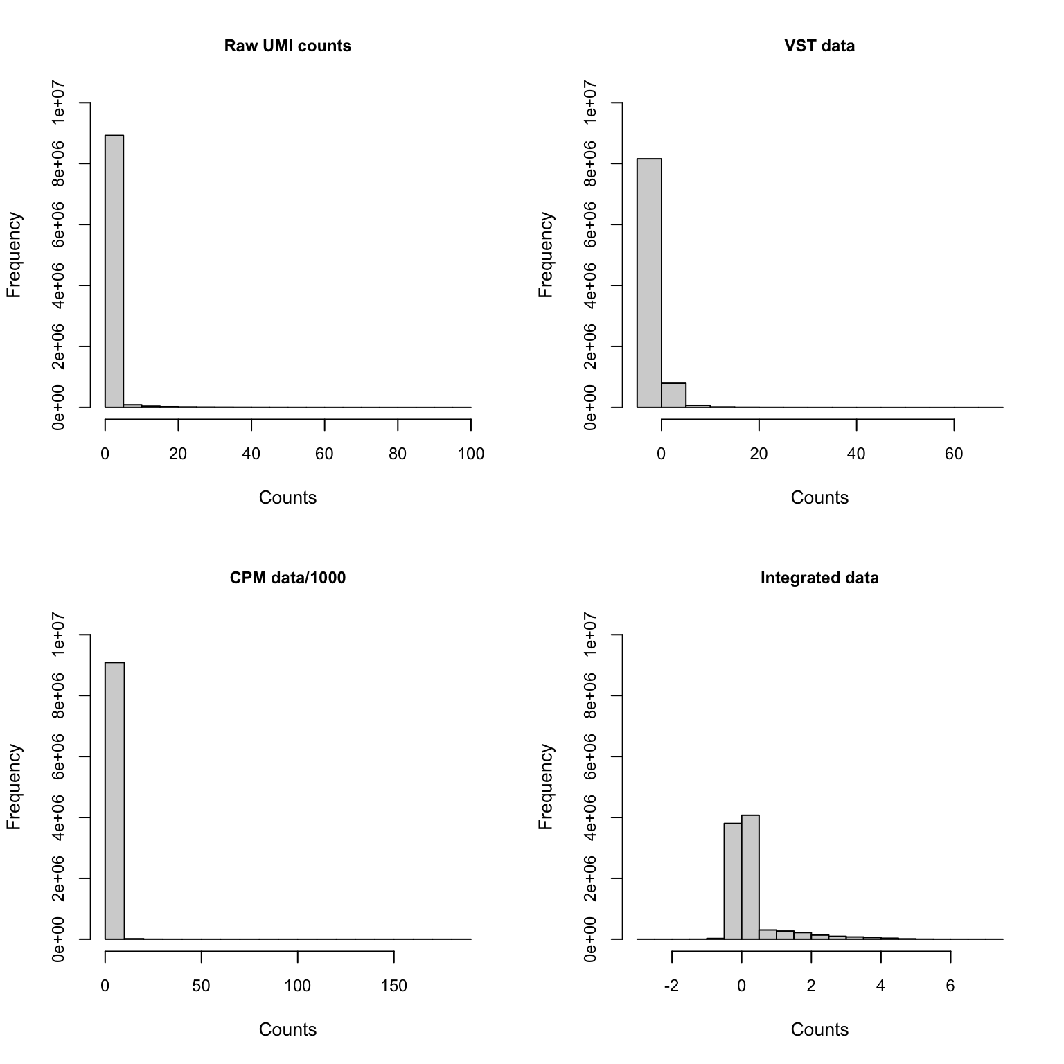
Version	Author	Date
e886219	C-HW	2024-10-14

If we zoom in on the positive counts, we may observe different distributions for each dataset.

Past versions of unnamed-chunk-13-1.png

Version	Author	Date
e886219	C-HW	2024-10-14

VST distribution

Past versions of unnamed-chunk-14-1.png

Version	Author	Date
e886219	C-HW	2024-10-14

Integrated data distribution

Past versions of unnamed-chunk-15-1.png

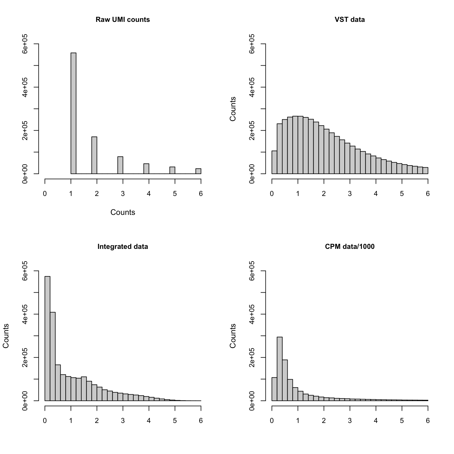
Version	Author	Date
e886219	C-HW	2024-10-14

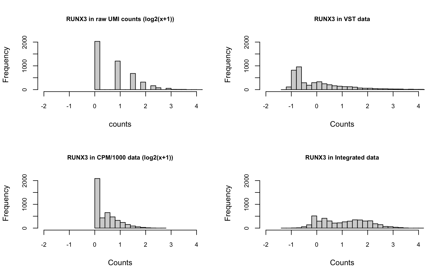
Single gene

We randomly choose one moderately expressed gene RUNX3. After normalization, the distribution of the counts changes a lot.

Past versions of unnamed-chunk-16-1.png

Version	Author	Date
e886219	C-HW	2024-10-14

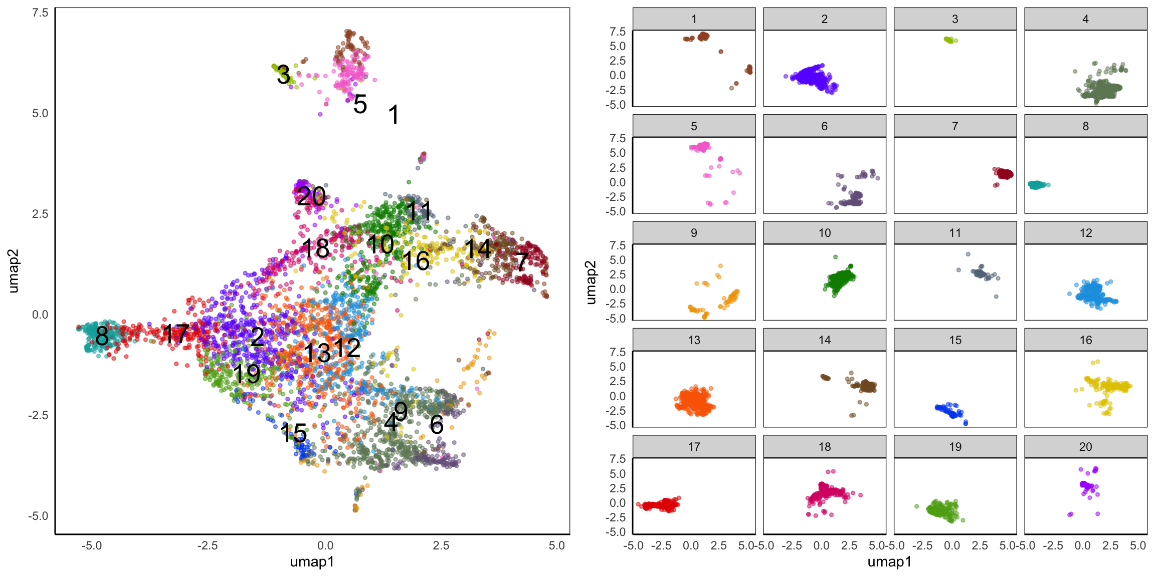
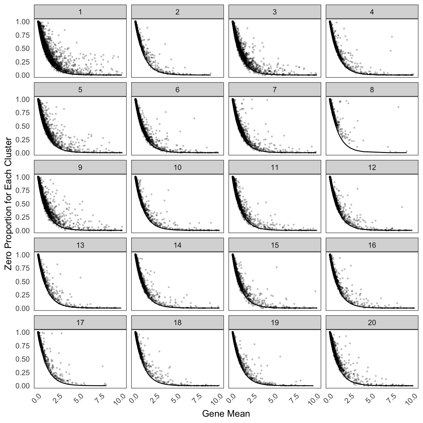
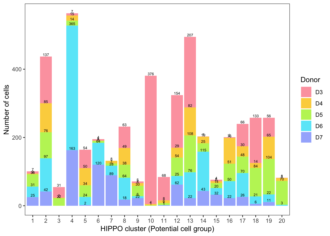
Hippo cluster result

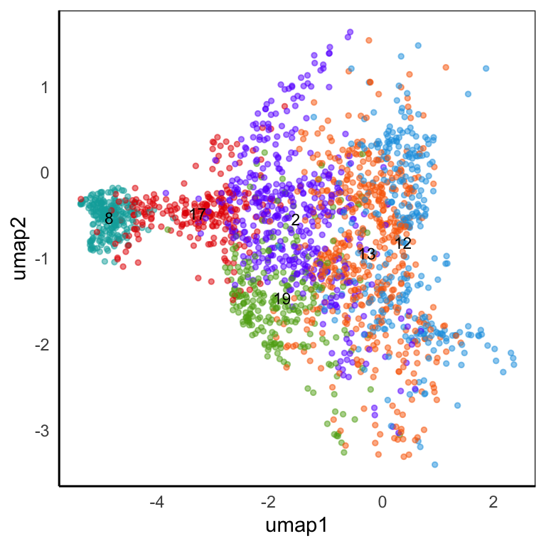
We applied HIPPO (Heterogeneity-Inspired Pre-Processing tOol) on the raw counts to get 20 clusters. Especially, cluster 2, 8, 12, 13, 17, 19 will be used to demonstrate our poisson glmm DE methods.

UMAP

Hippo procedure

Past versions of unnamed-chunk-21-1.png

Version	Author	Date
e886219	C-HW	2024-10-14

Interested groups

Past versions of unnamed-chunk-23-1.png

Version	Author	Date
e886219	C-HW	2024-10-14

Zero proportion plot

Past versions of unnamed-chunk-24-1.png

Version	Author	Date
e886219	C-HW	2024-10-14

Donor distribution

Past versions of unnamed-chunk-25-1.png

Version	Author	Date
e886219	C-HW	2024-10-14

Donor/Celltype/Residual variation

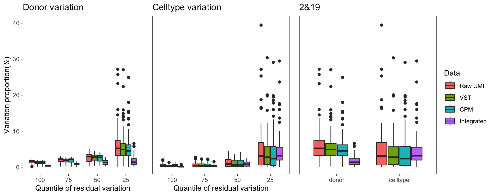
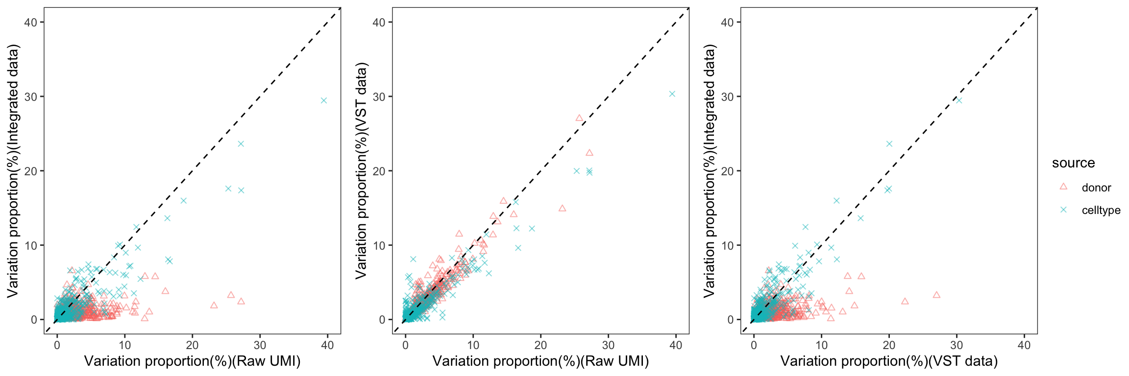
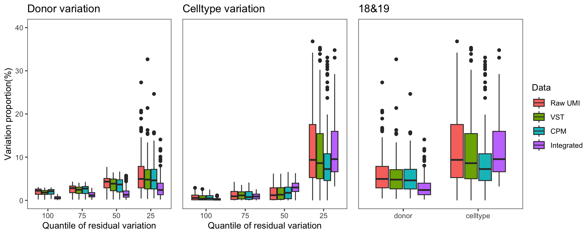
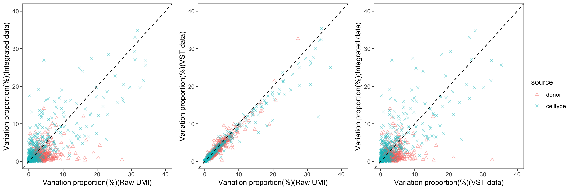
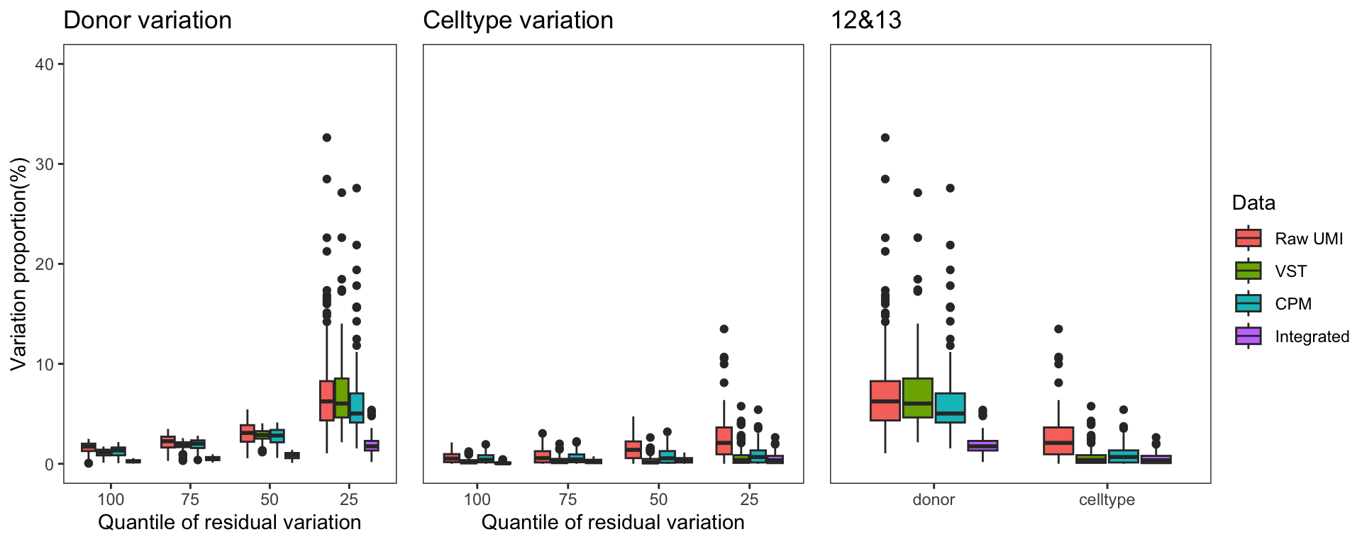
To gain a deeper understanding of the donor effect and cell type effect concerning various types of counts, we conducted a variation analysis across multiple group comparisons. To ensure the consistency of our results, we restricted our analysis to genes presented in all datasets. For each gene, we employed linear models (lm (count ~ donor + group)) and computed the variances attributed to three components: donor, group, and the residual. Logarithm transformation was applied to UMI counts and CPM data to address skewness.

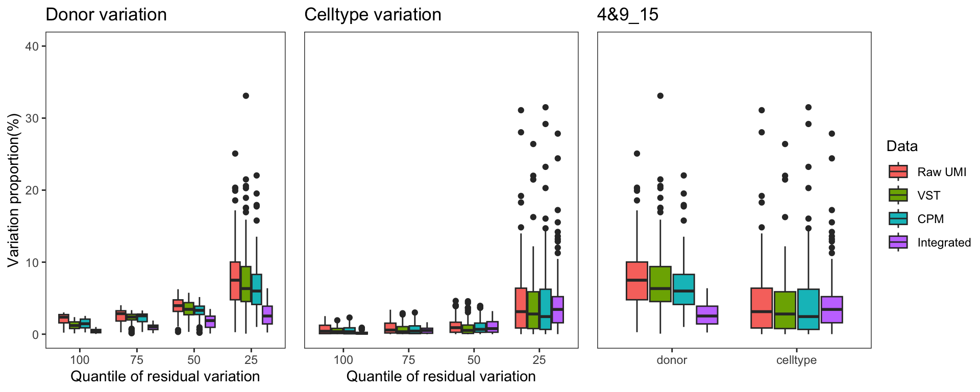
The following plots exhibit the top 500 genes with the lowest residual variations, showcasing the contributions of these variations as percentages. The genes were organized into bins based on the quantiles of residual variations. The last plot displays the first quartile and compare the donor variation and celltype variation

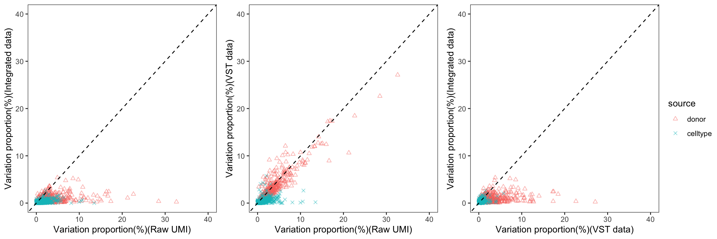
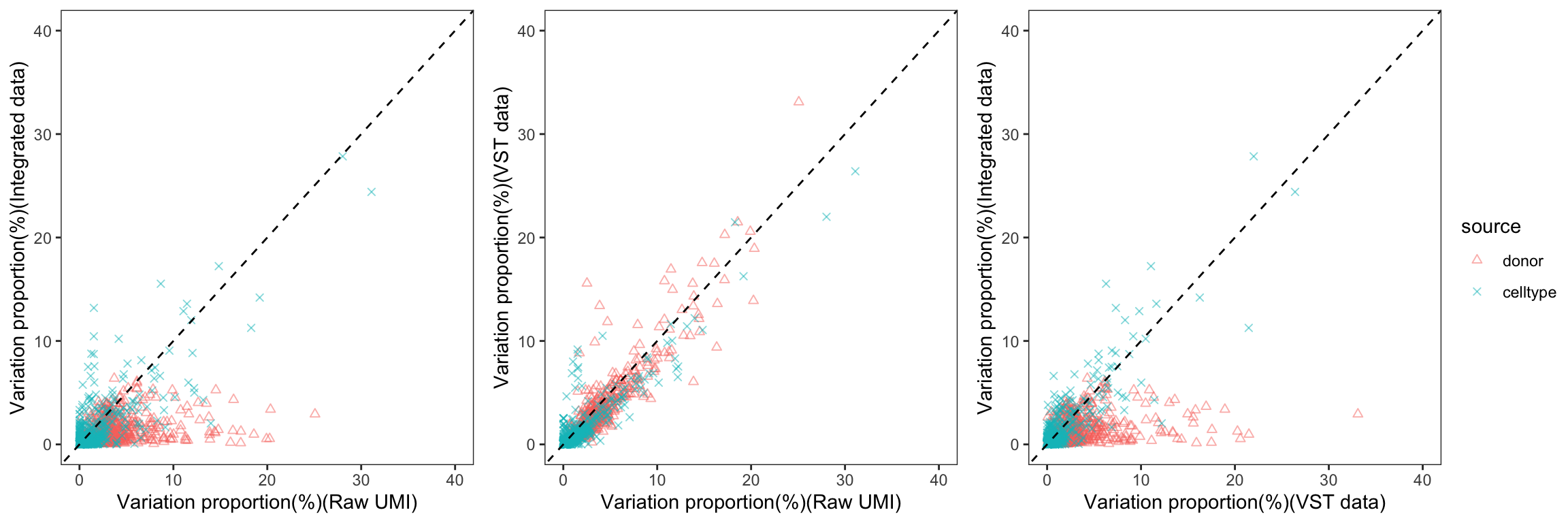
The integration of data did partially reduce the donor variations, although it did not eliminate them completely. However, it is worth noting that the normalization and batch effect removal processes employed also resulted in a reduction in celltype variation. This reduction in celltype variation may pose challenges for conducting further differential expression (DE) analysis.

Group 2, 19

Past versions of unnamed-chunk-28-1.png

Version	Author	Date
e886219	C-HW	2024-10-14

Past versions of unnamed-chunk-29-1.png

Version	Author	Date
e886219	C-HW	2024-10-14

Group 18, 19

Past versions of unnamed-chunk-31-1.png

Version	Author	Date
e886219	C-HW	2024-10-14

Past versions of unnamed-chunk-32-1.png

Version	Author	Date
e886219	C-HW	2024-10-14

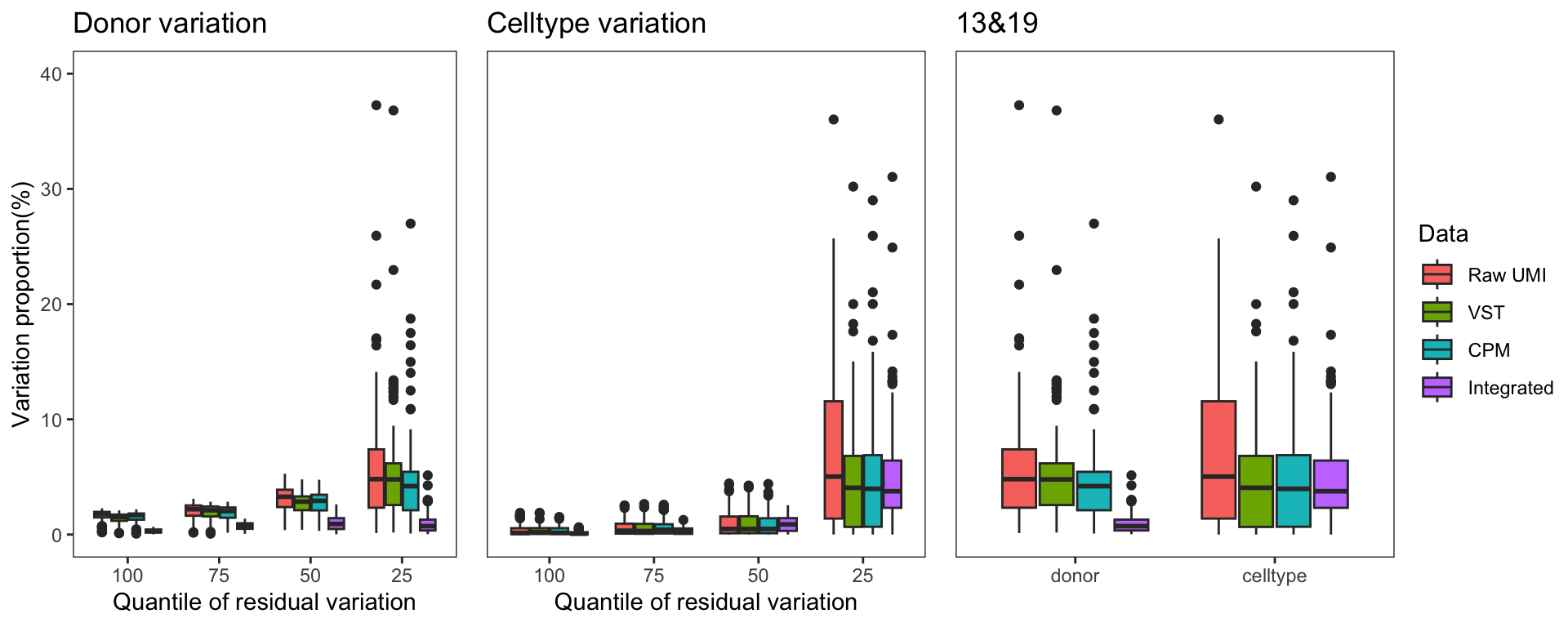
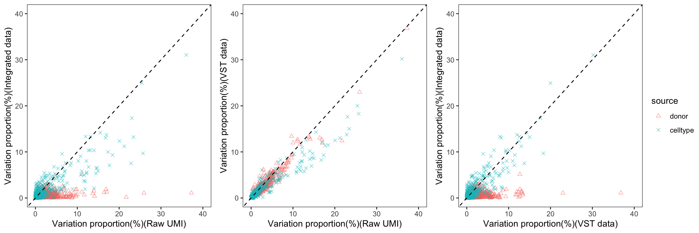
Group 13, 19

Past versions of unnamed-chunk-34-1.png

Version	Author	Date
e886219	C-HW	2024-10-14

Past versions of unnamed-chunk-35-1.png

Version	Author	Date
e886219	C-HW	2024-10-14

Group 12, 13

Past versions of unnamed-chunk-37-1.png

Version	Author	Date
e886219	C-HW	2024-10-14

Past versions of unnamed-chunk-38-1.png

Version	Author	Date
e886219	C-HW	2024-10-14

Group 4, 9&15

Past versions of unnamed-chunk-40-1.png

Version	Author	Date
e886219	C-HW	2024-10-14

Past versions of unnamed-chunk-41-1.png

Version	Author	Date
e886219	C-HW	2024-10-14

Session information

R version 4.4.1 (2024-06-14)
Platform: x86_64-apple-darwin20
Running under: macOS Monterey 12.6

Matrix products: default
BLAS:   /Library/Frameworks/R.framework/Versions/4.4-x86_64/Resources/lib/libRblas.0.dylib 
LAPACK: /Library/Frameworks/R.framework/Versions/4.4-x86_64/Resources/lib/libRlapack.dylib;  LAPACK version 3.12.0

locale:
[1] en_US.UTF-8/en_US.UTF-8/en_US.UTF-8/C/en_US.UTF-8/en_US.UTF-8

time zone: America/Chicago
tzcode source: internal

attached base packages:
[1] stats4    stats     graphics  grDevices utils     datasets  methods  
[8] base     

other attached packages:
 [1] Seurat_5.1.0                SeuratObject_5.0.2         
 [3] sp_2.1-4                    reshape2_1.4.4             
 [5] SingleCellExperiment_1.26.0 SummarizedExperiment_1.34.0
 [7] Biobase_2.64.0              GenomicRanges_1.56.2       
 [9] GenomeInfoDb_1.40.1         IRanges_2.38.1             
[11] S4Vectors_0.42.1            BiocGenerics_0.50.0        
[13] MatrixGenerics_1.16.0       matrixStats_1.4.1          
[15] ggpubr_0.6.0                dplyr_1.1.4                
[17] ggplot2_3.5.1              

loaded via a namespace (and not attached):
  [1] RColorBrewer_1.1-3      rstudioapi_0.16.0       jsonlite_1.8.9         
  [4] magrittr_2.0.3          spatstat.utils_3.1-0    farver_2.1.2           
  [7] rmarkdown_2.28          fs_1.6.4                zlibbioc_1.50.0        
 [10] vctrs_0.6.5             ROCR_1.0-11             spatstat.explore_3.3-2 
 [13] rstatix_0.7.2           htmltools_0.5.8.1       S4Arrays_1.4.1         
 [16] broom_1.0.7             SparseArray_1.4.8       Formula_1.2-5          
 [19] sctransform_0.4.1       sass_0.4.9              parallelly_1.38.0      
 [22] KernSmooth_2.23-24      bslib_0.8.0             htmlwidgets_1.6.4      
 [25] ica_1.0-3               plyr_1.8.9              plotly_4.10.4          
 [28] zoo_1.8-12              cachem_1.1.0            whisker_0.4.1          
 [31] igraph_2.0.3            mime_0.12               lifecycle_1.0.4        
 [34] pkgconfig_2.0.3         Matrix_1.7-0            R6_2.5.1               
 [37] fastmap_1.2.0           GenomeInfoDbData_1.2.12 fitdistrplus_1.2-1     
 [40] future_1.34.0           shiny_1.9.1             digest_0.6.37          
 [43] colorspace_2.1-1        patchwork_1.3.0         tensor_1.5             
 [46] rprojroot_2.0.4         RSpectra_0.16-2         irlba_2.3.5.1          
 [49] labeling_0.4.3          progressr_0.14.0        spatstat.sparse_3.1-0  
 [52] fansi_1.0.6             polyclip_1.10-7         httr_1.4.7             
 [55] abind_1.4-8             compiler_4.4.1          withr_3.0.1            
 [58] backports_1.5.0         carData_3.0-5           fastDummies_1.7.4      
 [61] highr_0.11              ggsignif_0.6.4          MASS_7.3-61            
 [64] DelayedArray_0.30.1     tools_4.4.1             lmtest_0.9-40          
 [67] httpuv_1.6.15           future.apply_1.11.2     goftest_1.2-3          
 [70] glue_1.8.0              nlme_3.1-166            promises_1.3.0         
 [73] grid_4.4.1              Rtsne_0.17              cluster_2.1.6          
 [76] generics_0.1.3          spatstat.data_3.1-2     gtable_0.3.5           
 [79] tidyr_1.3.1             data.table_1.16.2       car_3.1-3              
 [82] utf8_1.2.4              XVector_0.44.0          spatstat.geom_3.3-3    
 [85] RcppAnnoy_0.0.22        ggrepel_0.9.6           RANN_2.6.2             
 [88] pillar_1.9.0            stringr_1.5.1           spam_2.11-0            
 [91] RcppHNSW_0.6.0          later_1.3.2             splines_4.4.1          
 [94] lattice_0.22-6          deldir_2.0-4            survival_3.7-0         
 [97] tidyselect_1.2.1        pbapply_1.7-2           miniUI_0.1.1.1         
[100] knitr_1.48              git2r_0.33.0            gridExtra_2.3          
[103] scattermore_1.2         xfun_0.48               stringi_1.8.4          
[106] UCSC.utils_1.0.0        lazyeval_0.2.2          workflowr_1.7.1        
[109] yaml_2.3.10             evaluate_1.0.1          codetools_0.2-20       
[112] tibble_3.2.1            cli_3.6.3               uwot_0.2.2             
[115] xtable_1.8-4            reticulate_1.39.0       munsell_0.5.1          
[118] jquerylib_0.1.4         Rcpp_1.0.13             spatstat.random_3.3-2  
[121] globals_0.16.3          png_0.1-8               spatstat.univar_3.0-1  
[124] parallel_4.4.1          dotCall64_1.2           listenv_0.9.1          
[127] viridisLite_0.4.2       scales_1.3.0            ggridges_0.5.6         
[130] leiden_0.4.3.1          purrr_1.0.2             crayon_1.5.3           
[133] rlang_1.1.4             cowplot_1.1.3